SDOF hysteresis – Models A, B, and C
Single-degree-of-freedom oscillator with prescribed harmonic displacement \(u(t) = u_0 \sin(\omega t)\). This page explains three common damping idealizations and shows how they affect the force–displacement loop shape, the energy dissipated per cycle, and the effective stiffness felt by the structure.
Key questions this page answers
The visualizations and formulas below are organized to answer four practical questions:
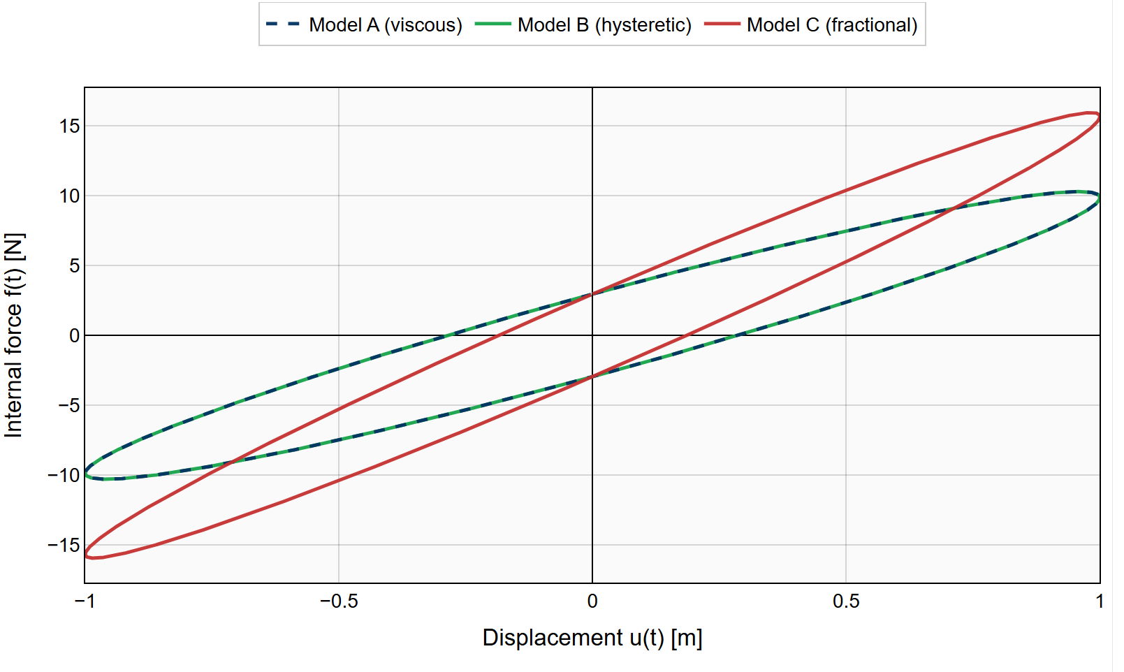
- How do different damping models change the hysteresis loop? We compare the force–displacement loops of three models for the same imposed motion.
- How much energy is dissipated per cycle? We compute the loop area (EDC) numerically and track how it varies with loading frequency.
- What do “storage” and “loss” stiffness mean? We introduce \(K_1\) and \(K_2\) as in‑phase and out‑of‑phase stiffness, linked to loop tilt and area.
- When is a fractional model useful? We show how the fractional Kelvin–Voigt model can interpolate between purely viscous and purely hysteretic behavior.
Problem setting and notation
The analysis is performed in relative coordinates \(u(t)\) (m), with internal resisting force \(f(t)\) (N). The internal force is decomposed as \(f(t) = f_r(t) + f_d(t)\), where:
- \(f_r(t) = k\,u(t)\) is the elastic restoring force, with stiffness \(k\) (N/m).
- \(f_d(t)\) is the dissipative force, specified by the damping model.
The baseline parameters are: \[ m = 1~\mathrm{kg},\qquad \omega_n = \pi~\mathrm{rad/s},\qquad k = m\omega_n^2 = \pi^2~\mathrm{N/m}. \]
In Part (a), the displacement is prescribed in steady state as \[ u(t) = u_0 \sin(\omega t),\qquad u_0 = 1~\mathrm{m}, \] with circular frequency \(\omega\) (rad/s). One cycle has duration \(T = 2\pi/\omega\). The hysteresis loop is the parametric curve \(\bigl(u(t), f(t)\bigr)\) for \(t \in [0, T]\). Its enclosed area equals the closed-loop work \(\mathrm{EDC} = \oint f\,du\) (J), representing the energy dissipated per cycle, while the overall tilt of the loop reflects the in-phase stiffness that stores recoverable strain energy.
Harmonic decomposition and dynamic stiffness
For the imposed motion \(u(t) = u_0 \sin(\omega t)\) with \(\dot{u}(t) = u_0 \omega \cos(\omega t)\), any linear model produces a steady-state force at the same frequency that can be written uniquely as \[ f(t) = K_1(\omega)\,u_0 \sin(\omega t) + K_2(\omega)\,u_0 \cos(\omega t), \] which defines:
- \(K_1(\omega)\) (N/m): storage stiffness, multiplying the in-phase term \(\sin(\omega t)\),
- \(K_2(\omega)\) (N/m): loss stiffness, multiplying the quadrature term \(\cos(\omega t)\), in phase with \(\dot{u}(t)\).
Introducing the complex dynamic stiffness \[ \hat{R}(\omega) = K_1(\omega) + \mathrm{i}K_2(\omega),\qquad F(\omega) = \hat{R}(\omega)\,U(\omega), \] aligns this time-domain decomposition with the Fourier-domain representation, where \(U(\omega)\) and \(F(\omega)\) are the Fourier transforms of \(u(t)\) and \(f(t)\). For real-valued time histories the spectra satisfy \[ U(-\omega) = \overline{U(\omega)},\qquad F(-\omega) = \overline{F(\omega)}, \] which implies the conjugate-symmetry requirement \(\hat{R}(-\omega) = \overline{\hat{R}(\omega)}\). This condition is enforced explicitly in the frequency-domain forms of Models B and C in the earthquake-response scripts by using \(\operatorname{sgn}(\omega)\).
Damping models under prescribed motion
-
Model A – Kelvin–Voigt (viscous)
Constitutive law: \[ f(t) = k\,u(t) + c\,\dot{u}(t), \] with viscous coefficient \(c\) (N·s/m). For the imposed motion, \[ f(t) = k\,u_0 \sin(\omega t) + (c\omega)\,u_0 \cos(\omega t), \] so \[ K_1^{(A)}(\omega) = k,\qquad K_2^{(A)}(\omega) = c\omega. \] In the frequency domain, \[ \hat{R}^{(A)}(\omega) = k + \mathrm{i}c\omega, \] which automatically satisfies \(\hat{R}^{(A)}(-\omega) = \overline{\hat{R}^{(A)}(\omega)}\). -
Model B – hysteretic (structural, harmonic idealization)
Harmonic idealization: \[ f(t) = k\,u_0 \sin(\omega t) + k\delta\,u_0 \cos(\omega t), \] with loss factor \(\delta\) (dimensionless). Comparison with the decomposition gives \[ K_1^{(B)}(\omega) = k,\qquad K_2^{(B)}(\omega) = k\delta, \] so the loop area and energy dissipated per cycle are independent of \(\omega\). For two-sided spectra, a frequency-domain implementation uses \[ \hat{R}^{(B)}(\omega) = k\Bigl(1 + \mathrm{i}\delta\,\operatorname{sgn}(\omega)\Bigr), \] which enforces \(\hat{R}^{(B)}(-\omega) = \overline{\hat{R}^{(B)}(\omega)}\). -
Model C – fractional Kelvin–Voigt
Constitutive law: \[ f(t) = k\,u(t) + c_\alpha D^\alpha u(t),\qquad 0 < \alpha < 1, \] where \(c_\alpha\) (N·s\(^{-\alpha}\)/m) is a material constant and \(D^\alpha\) denotes a linear fractional-derivative operator of order \(\alpha\). For harmonic motion the identity \[ D^\alpha[\sin(\omega t)] = \omega^\alpha \sin\!\left(\omega t + \frac{\pi\alpha}{2}\right) \] leads to \[ K_1^{(C)}(\omega) = k + c_\alpha \omega^\alpha \cos\!\left(\frac{\pi\alpha}{2}\right),\qquad K_2^{(C)}(\omega) = c_\alpha \omega^\alpha \sin\!\left(\frac{\pi\alpha}{2}\right). \] The same fractional element therefore adds both a storage contribution \(\Delta K_1\) and a loss contribution \(\Delta K_2\), which is why matching dissipation (loop area) at a target frequency generally changes the loop tilt unless the elastic term in Model C is adjusted.
Hysteresis loops at resonance (ω = ωₙ)
Force–displacement hysteresis loops for the three models at \(\omega = \omega_n\). All loops share the same elastic stiffness \(k\), but differ in how dissipation is introduced and how the loss stiffness \(K_2(\omega)\) depends on frequency. At \(\omega = \omega_n\), the parameters are chosen so that Models A and B have identical \((K_1, K_2)\), and Model C is calibrated to match the same \(\mathrm{EDC}(\omega_n)\). The overlay highlights how the fractional model can reproduce the loop area while still exhibiting a different tilt if the elastic term is not further adjusted.
Energy dissipated per cycle vs frequency
The energy dissipated per cycle is defined geometrically as the loop area \(\mathrm{EDC} = \oint f\,du\) in the \((u,f)\) plane. In this dashboard it is evaluated numerically by integrating the simulated loop for each model.
For each frequency \(\omega\) in the range \(0.5\,\omega_n \le \omega \le 2\,\omega_n\), one full cycle \(T = 2\pi / \omega\) is sampled finely in time. The prescribed displacement \(u(t)\) and the corresponding force \(f(t)\) are computed for each model, the loop is explicitly closed by appending the starting point, and the area is obtained from a polygonal (polyarea‑style) formula in the \((u,f)\) plane.
The resulting \(\mathrm{EDC}(\omega)\) curves match the analytic identity \(\mathrm{EDC}(\omega) = \pi K_2(\omega) u_0^2\) and make the frequency dependence of dissipation clear: viscous damping grows approximately linearly with \(\omega\), the hysteretic idealization is nearly constant, and the fractional model exhibits intermediate \(\omega^\alpha\) behavior.
Model A (viscous) grows approximately linearly with \(\omega\), Model B (hysteretic idealization) is frequency independent, and Model C (fractional) exhibits intermediate \(\omega^\alpha\) dependence. At \(\omega = \omega_n\), all three curves intersect by construction, confirming equal \(\mathrm{EDC}\) at resonance.
Storage and loss stiffness, and energy per cycle at ω = ωₙ
The table below lists the analytical storage stiffness \(K_1(\omega_n)\), loss stiffness \(K_2(\omega_n)\), and energy dissipated per cycle \(\mathrm{EDC}(\omega_n)\) for \(u_0 = 1\). Stiffnesses are given in N/m and \(\mathrm{EDC}\) in N·m (J).
| Model | \(K_1(\omega_n)\) | \(K_2(\omega_n)\) | \(\mathrm{EDC}(\omega_n)\) |
|---|---|---|---|
| Model A (viscous) | 9.8696 | 2.9609 | 9.3019 |
| Model B (hysteretic) | 9.8696 | 2.9609 | 9.3019 |
| Model C (fractional) | 15.6823 | 2.9617 | 9.3045 |
Earthquake response via frequency-domain analysis
In relative coordinates \(u(t)\), the SDOF balance under base excitation is \[ m u''(t) + f_d(t) + k\,u(t) = -m\,\ddot{u}_g(t), \] where \(f_d(t)\) is the model-dependent damping force and \(\ddot{u}_g(t)\) is the ground acceleration. Introducing the dynamic stiffness \(\hat{R}(\omega)\) such that \(F(\omega) = \hat{R}(\omega) U(\omega)\), Fourier transforming gives \[ \bigl(\hat{R}(\omega) - m\omega^2\bigr)U(\omega) = -m\,\ddot{U}_g(\omega), \qquad U(\omega) = H(\omega)\,\ddot{U}_g(\omega),\quad H(\omega) = -\frac{m}{\hat{R}(\omega) - m\omega^2}. \]
For each damping model, the appropriate \(\hat{R}(\omega)\) is used: Model A: \(\hat{R}^{(A)}(\omega) = k + i c \omega\); Model B: \(\hat{R}^{(B)}(\omega) = k\bigl(1 + i\delta\,\operatorname{sgn}(\omega)\bigr)\); Model C: \(\hat{R}^{(C)}(\omega) = k_C + c_\alpha (i\omega)^\alpha\) with the two-sided fractional power ensuring conjugate symmetry. The spectra \(U(\omega)\), \(V(\omega) = i\omega U(\omega)\), and \(\ddot{U}_{\mathrm{abs}}(\omega)\) are computed using NumPy's FFT routines and transformed back to the time domain via inverse FFT to obtain the displacement, velocity, and absolute acceleration responses under the Kobe KBU090 motion.
The figure below compares the three models on a common time axis. Because the FFT method treats long records efficiently and makes the frequency dependence of \(\hat{R}(\omega)\) explicit, it is well suited to this comparison; however, it also relies on linearization and periodic extension of the record, so care is needed when interpreting results for strongly nonlinear behavior or for motions with significant trends.